Having worked through Andrej Karpathy’s fantastic makemore series, I want to implement some recent advances in transformers to gain deeper understanding. Inspired by the style of makemore, this series of posts will in a progressive approach, implementing minimal versions of advanced transformer features for learning purposes.
Here’s a preview of the key features of modern transformers I’d like to cover in a series of posts:
- Part 1: SwiGLU
- Part 2: Rotary Positional Embedding (RoPE)
- Part 3: Grouped-query attention (GQA)
I aim not only to demonstrate how to implement these improvements in PyTorch but also to intuitively explain the problems they solve. Let’s begin by setting up a minimal GPT baseline.
import pandas as pd
from tqdm import tqdm

import torch
import torch.nn as nn
from torch.nn import functional as F

torch.manual_seed(42)
Introduction
MinGPT with Multi-head Attention
Following Let’s build GPT, we should have ended up with a Multi-head attention (MHA) implementation resembling the following:
class MultiHeadAttention(nn.Module):
    def __init__(self, num_heads) -> None:
        super().__init__()
        self.attn = nn.Linear(embed_size, 3 * embed_size, bias=False)
        self.register_buffer(
            "tril",
            torch.tril(torch.ones(context_size, context_size)).view(
                1, 1, context_size, context_size
            ),
        )
        self.attn_dropout = nn.Dropout(dropout)
        self.rsid_dropout = nn.Dropout(dropout)
        self.proj = nn.Linear(embed_size, embed_size)
        self.num_heads = num_heads

    def forward(self, x):
        B, C, E = x.size() # B for batch size, C for context size, E for embed size
        NH = self.num_heads # NH for number of heads
        attn_out = self.attn(x)  # (B,C,E) --> (B,C,3E)
        k, q, v = attn_out.split(embed_size, dim=2)  # (B,C,E)
        k = k.view(B, C, NH, E // NH).transpose(
            1, 2
        )  # (B,C,NH,HS) --> (B,NH,C,HS) # HS for head size
        q = q.view(B, C, NH, E // NH).transpose(1, 2)
        v = v.view(B, C, NH, E // NH).transpose(1, 2)
        wei = (
            q @ k.transpose(-2, -1) * (E // NH) ** -0.5
        )  # (B,NH,C,HS) @ (B,NH,HS,C) --> (B,NH,C,C)
        wei = wei.masked_fill(self.tril[:, :, :C, :C] == 0, float("-inf"))
        wei = F.softmax(wei, dim=-1)
        wei = self.attn_dropout(wei)  # (B,NH,C,C)
        out = wei @ v  # (B,NH,C,C) @ (B,NH,C,HS) --> (B,NH,C,HS)
        out = (
            out.transpose(1, 2).contiguous().view(B, C, E)
        )  # concat --> (B,C,E) where E is NH*HS
        proj_out = self.rsid_dropout(self.proj(out))  # (B,C,E)
        return proj_out
Here, num_heads represents the number of attention heads, embed_size denotes the hidden or embedding size, and context_size is our context length. Notably, the module processes multiple attention heads in a single forward pass, assuming our embedding size is a multiple of the number of heads. This aligns with the GPT attention design. For example, GPT-2 small has an embedding size of 768 and 12 heads, resulting in a head size of 64. I have written clear comments for each transformation in the forward pass, but for a clearer visualization, refer to Jay Alammar’s insightful post.
GPT’s decoder-only architecture is essentially a stacking of MHA blocks containing MHA modules and feed-forward layers with activation nonlinearities and layer normalizations.
class FeedForward(nn.Module):
    def __init__(self, embed_size) -> None:
        super().__init__()
        self.net = nn.Sequential(
            nn.Linear(embed_size, 4 * embed_size, bias=False),  # scale hidden size
            nn.ReLU(),
            nn.Linear(4 * embed_size, embed_size, bias=False),
            nn.Dropout(dropout),
        )

    def forward(self, x):
        return self.net(x)


class Block(nn.Module):
    def __init__(self, embed_size, num_heads) -> None:
        super().__init__()
        self.mha = MultiHeadAttention(num_heads)
        self.ffwd = FeedForward(embed_size)
        self.ln_mha = nn.LayerNorm(embed_size)
        self.ln_ff = nn.LayerNorm(embed_size)

    def forward(self, x):
        x = x + self.mha(self.ln_mha(x)) # pre-norm
        x = x + self.ffwd(self.ln_ff(x))
        return x


class MinGPT(nn.Module):

    def __init__(self):
        super().__init__()
        self.token_embedding_table = nn.Embedding(vocab_size, embed_size)
        self.positional_embedding_table = nn.Embedding(context_size, embed_size)
        self.blocks = nn.Sequential(
            *[Block(embed_size, num_heads) for _ in range(n_layer)]
        )
        self.ln_f = nn.LayerNorm(embed_size)
        self.lm_head = nn.Linear(embed_size, vocab_size)

    def forward(self, idx, targets=None):
        B, C = idx.shape
        tok_emb = self.token_embedding_table(idx)  # (B,C,E)
        pos_emb = self.positional_embedding_table(
            torch.arange(C, device=device)
        )  # (C,E)
        x = tok_emb + pos_emb
        x = self.blocks(x)
        x = self.ln_f(x)
        logits = self.lm_head(x)

        if targets is None:
            loss = None
        else:
            B, C, E = (
                logits.shape
            )  # B for batch size, C for context size, E for embed size
            logits = logits.view(B * C, E)
            targets = targets.view(B * C)
            loss = F.cross_entropy(logits, targets)

        return logits, loss
Training Data
Up to this point, everything should be familiar from makemore. One of the suggested exercises from Let’s build GPT involves training it to perform simple calculations. Thus, I thought it would be opportune to train our own GPT calculator, exploring each improvement’s impact on its arithmetic capabilities.
For this purpose, I generated a training dataset and testing dataset of math problems involving simple operations (addition, subtraction, multiplication, division) on numbers within the range of (0,1000]. Each question was converted to a string, padded with zeros to match length, and the answer was reversed. I used ‘$’ instead of the usual
$(0000753.78+0000000910)=87.3661000$
$(0000000782+0000000021)=3080000000$
$(0000002.08-0000136.22)=41.431-000$
$(0000313.46*0000000217)=28.0208600$
$(0000000573*0000351.77)=12.4651020$
$(0000000400/0000000344)=61.1000000$
$(0000000471/0000000299)=85.1000000$
The code used to generate these questions (training dataset of 3M questions and testing dataset of 10k questions) can be found here. Feel free to use the script to generate more complex problems. Additionally, for comparison, we’ll train a separate model with the [TinyShakespeare] dataset, providing insights into the model’s performance variations with different data.
To train our MinGPT on the math dataset, we’ll utilize the same character-level tokenizer as in makemore. The following code reads in the training data, builds our character-to-index encoder and index-to-character decoder, and consolidates the math problems into a single string for training-validation splits. This processing yields a vocab_size of 21 for the math problems dataset and 65 for TinyShakespeare.
with open("./data/train.txt", "r", encoding="utf-8") as f:
    text = f.read()
    text = "".join(text.split("\n")) # not for TinyShakespeare

chars = sorted(list(set(text)))
vocab_size = len(chars)

# encoder: character to index, decoder: index to character
stoi = {ch: i for i, ch in enumerate(chars)}
itos = {i: ch for i, ch in enumerate(chars)}
encode = lambda s: [stoi[c] for c in s]
decode = lambda l: "".join([itos[i] for i in l])

# Train and test splits at 90%
data = torch.tensor(encode(text), dtype=torch.long)
n = int(0.9 * len(data))
train_data = data[:n]
val_data = data[n:]
Baseline Training and Results
With the dataset prepared, we can now define hyperparameters for the model and begin training. To keep computational load low, we’ll opt for a small model and train for 5000 steps. The code for training and estimating loss is identical to that in makemore, and can be found in the baseline file here. Notice here that we did not apply dropout during training.
batch_size = 16
context_size = 128
max_iters = 5000
eval_interval = 500
learning_rate = 3e-4
device = "cuda" if torch.cuda.is_available() else "cpu"
eval_iters = 200
embed_size = 96
num_heads = 8  # head_size = 96/8 = 12
n_layer = 8
dropout = 0.0
The training and validation loss of the model trained on TinyShakespeare reveal the potential for overfitting with our model size. However, while there are unseen variations in math problems in the validation set, there shouldn’t be any unseen patterns within them, hence the very close training and validation losses.
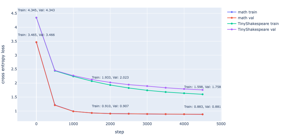
Our math dataset allows us to extrinsically evaluate the model’s ability to perform simple math operations through the test set:
with open("./data/test.txt", "r", encoding="utf-8") as f:
    testset = f.read()
    testset = testset.split("\n") # split to problems

preds = []
y = []

for i in range(len(testset)):
    # for each problem, such as "$(0000000585*0000165.64)=", provide as context to sample from model
    t = f'{testset[i].split("=")[0]}='
    context = torch.tensor(encode(t), dtype=torch.long, device=device)
    idx = context.view((1, len(context)))
    # sample until '$' emitted
    while True:
        idx_cond = idx[:, -context_size:]
        logits, loss = baseline_model(
            idx_cond
        )  # baseline model trained on math dataset
        logits = logits[:, -1, :]
        probs = F.softmax(logits, dim=-1)
        idx_next = torch.multinomial(probs, num_samples=1)
        if idx_next.item() == 0:
            idx = torch.cat((idx, idx_next), dim=1)
            break
        idx = torch.cat((idx, idx_next), dim=1)

    # trim if pred too long, pad if too short
    gtruth = torch.tensor(encode(testset[i]), dtype=torch.long)
    y.append(gtruth)
    if len(idx[0]) < len(gtruth):
        pred = F.pad(idx[0], (0, len(gtruth) - len(idx[0])), "constant", 0)
    else:
        pred = idx[0][: len(gtruth)]
    preds.append(pred)

# stack predictions
preds = torch.stack(preds, dim=0)
y = torch.stack(y, dim=0)
With the predictions, we can evaluate the accuracy of the ‘calculations’. Furthermore, since they are ‘calculations’, we should evaluate exact match as well:
# get index of '=' in problem
eql = encode('=')[0]
eql_idx = (y[0] == eql).nonzero(as_tuple=True)[0].item()
# evaluate only predictions, ie, after '='
acc_preds = preds[:, eql_idx + 1 :]
acc_y = y[:, eql_idx + 1 :]

# accuracy
accuracy = (acc_preds == acc_y).sum().item() / float(
    acc_preds.shape[0] * acc_preds.shape[1]
) # 0.592872

# exact match
em = (acc_preds == acc_y).all(dim=1).sum().item() / float(acc_preds.shape[0]) # 0.0007
Here, our math model achieved an accuracy of 0.5928 and a somewhat laughable EM of 0.0007 on the testing data. Perhaps for the sake of correctness, we shouldn’t use this model as our calculator just yet.
With the baseline established, let’s delve into how we might improve upon it with more modern activation functions.
Activation Functions
Why not ReLU?

The dying ReLU problem is a well-known issue with ReLU, which is defined as:
$$ ReLU(x) = max(0,x) $$any dead neuron outputs the same value for any input, and gradient descent does not update the weights. In other words, the neuron effectively does not learn and does not contribute to discerning the predictions. Based solely on the function above, we might wonder why ReLU works so well and dying ReLU is not a bigger issue considering any negative input will result in 0 gradient. In fact, let us simplify our feedforward layer and visualize the ReLU output of a random tensor:
ex = torch.randn(context_size, embed_size) # random example
normed = nn.LayerNorm(embed_size)(ex) # pre-norm

class FeedForward(nn.Module):
    def __init__(self, embed_size) -> None:
        super().__init__()
        self.net = nn.Sequential(
            nn.Linear(embed_size, embed_size, bias=False),
            nn.ReLU(),
        )

    def forward(self, x):
        return self.net(x)

ff = FeedForward(embed_size)
out = ff(normed).detach().numpy()
plt.imshow((out == 0.0))
plt.colorbar()
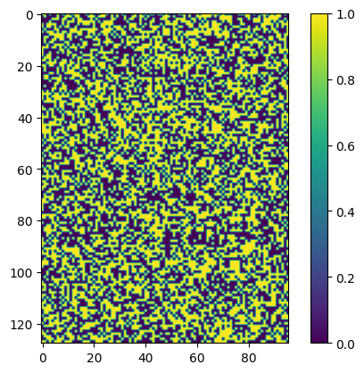
Notice that a significant portion of the outputs is 0. ReLU’s effectiveness in practice stems from the optimizer algorithm considering multiple inputs to the network. In the case of stochastic gradient descent, the algorithm will evaluate the gradient of the mini-batch data. Thus as long as one of the input has a non-zero gradient, the neuron weights will update and the network learns. Conversely, if all of the inputs have zero gradient, the neuron is “dead”.
Another issue with ReLU is in its bias shift. As Andrej illustrated very clearly in Building makemore, maintaining a roughly normal distribution in activation is crucial for well-behaved gradient updates. Normalization layers such as BatchNorm and LayerNorm significantly resolve this issue. In our model, pre-normalization is applied before the MHA output enters the first linear layer. But what happens to the output of the ReLU activation? Refer to the activation image above; what are the mean and variance of the ReLU activation output?
# Define an random example tensor
example_tensor = torch.randn(3, 3, dtype=torch.float32)
# norm
example_tensor = nn.LayerNorm(3)(example_tensor)

# Apply ReLU activation function
relu_tensor = F.relu(example_tensor)

# Calculate mean and variance before and after applying ReLU
mean_before = example_tensor.mean()
variance_before = example_tensor.var()
mean_after = relu_tensor.mean()
variance_after = relu_tensor.var()

print(f"Mean before: {mean_before.item():.4f}, Mean after: {mean_after.item():.4f}")
print(f"Variance before: {variance_before.item():.4f}, Variance after: {variance_after.item():.4f}")

# Mean before: 0.0000, Mean after: 0.4306
# Variance before: 1.1247, Variance after: 0.4179
Notice the positive shift in mean values and a reduction in variance for the output of ReLU for a random tensor normalized by layer. This attribute of the ReLU function results from its positive-only activation. When activations with a positive mean do not cancel out, a positive bias shift passes to the next layer. Clevert et al. demonstrated that reducing bias shift speeds up learning and recommended “(i) activation of incoming units can be centered at zero or (ii) activation functions with negative values can be used” to mitigate undesired bias shift effects.
SwiGLU
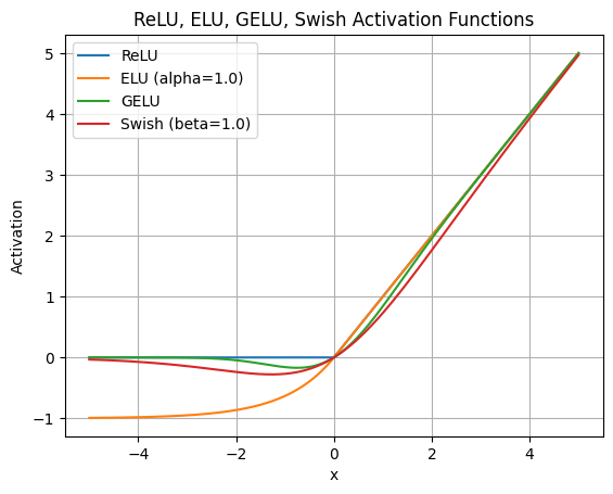
Various attempts have been made to replace ReLU with different activation functions, such as Exponential Linear Units [Clevert et al., 2016], Gaussian Error Linear Units [Hendrycks et al., 2016], and Swish [Ramachandran et al., 2017]. Initialization procedures were even developed to mitigate the dying ReLU problem [Lu et al., 2019].
In 2016, Dauphin et al. introduced Gated Linear Units (GLUs) in their attempt to apply convolutional neural networks for language modeling. Instead of applying regular ReLU or Tanh functions for activations, their network passes the previous tensor through separate linear layers and applies sigmoid to only one layer output before combining the outputs with element-wise multiplication:
$$ GLU(x) = \sigma(xW+b) \otimes (xV+c) $$where \(\mathnormal{W}\), \(\mathnormal{b}\) and \(\mathnormal{V}\), \(\mathnormal{c}\) are the weights and bias of the two linear layers, and \(\sigma\) is the sigmoid function. At this stage you might want to pause to wonder why GLU works well. Notice that GLU is not an activation function, but rather a network layer, as its name suggests.
Reveal
Intuitively it has to do with backpropagation and gradient flows, much like how Andrej spent a large portion of makemore explaining. In the two paths in which our loss has to backpropagate through, \(\sigma(xW+b)\) and \((xV+c)\), provides two gradient flows that adds up for \(x\). Dauphin et al. explains that for the path without activation, there is a "linear path that lets the gradient easily pass through", while the other path allows GLU to retain nonlinear capabilities provided by the activation. The authors also provided empirical results showing GLU outperforming ReLU for a faster convergence, contributing this effect to its "linear pass through".
SwiGLU, a GLU variant with the Swish activation instead of sigmoid, is expressed as:
$$ SwiGLU(x) = Swish_{\beta}(xW+b) \otimes (xV+c) $$where the $Swish$ activation as shown in the graph above, has the formula,
$$ Swish_{\beta} = x \sigma(\beta x) $$Here, \(\sigma\) is again the sigmoid function, and \(\beta\) is a trainable parameter. \(\beta\) is set to \(\mathnormal{1}\) to give \(\mathnormal{Swish_1}\), or just \(Swish\) as described in Ramachandran et al., 2017.
In GLU Variants Improve Transformer, 2020, Noam Shazeer proposed implementing these GLUs and their variants into the feedforward layers of the Transformer. GLU replaces the first linear layer and its activation. Specifically, the GLU and SwiGLU variants replace the feedforward layer with ReLU:
$$ FFN_{ReLU}(x, W_1, W_2) = max(xW_1, 0)W_2 $$With:
$$ FNN_{GLU}(x, W, V, W_2) = (\sigma(xW) \otimes xV)W_2 $$ $$ FNN_{SwiGLU}(x, W, V, W_2) = (SwiGLU(xW) \otimes xV)W_2 $$Empirical studies by Noam Shazeer demonstrated that these GLU variants outperform their non-GLU counterparts, suggesting a notable improvement in convergence speed.
SwiGLU has become a staple in modern architectures, implemented in foundation models from LLaMA2 to PaLM2. Let's implement it in PyTorch to enhance our model's performance. Replacing the \(FFN_{ReLU}\) layer with SwiGLU:class FeedForward(nn.Module):
def __init__(self, embed_size) -> None:
super().__init__()
self.net = nn.Sequential(
nn.Linear(embed_size, 4 * embed_size, bias=False), # scale hidden size
nn.ReLU(),
nn.Linear(4 * embed_size, embed_size, bias=False),
nn.Dropout(dropout),
)
def forward(self, x):
return self.net(x)
we now replace the first linear layer and the ReLU activation with SwiGLU,
class FeedForward(nn.Module):
    def __init__(self, embed_size: int) -> None:
        super().__init__()
        hidden_dim = int(2 * embed_size / 3) # scale hidden to match parameter count
        self.w = nn.Linear(embed_size, 4 * hidden_dim, bias=False)
        self.w2 = nn.Linear(4 * hidden_dim, embed_size, bias=False)
        self.v = nn.Linear(embed_size, 4 * hidden_dim, bias=False)
        self.dropout = nn.Dropout(dropout)

    def forward(self, x: torch.Tensor) -> torch.Tensor:
        return self.dropout(self.w2(F.silu(self.w(x)) * self.v(x)))
PyTorch’s F.silu corresponds to \(Swish_1\). Additionally, to ensure fair comparison, we scale the hidden dimension by a factor of \(\frac{2}{3}\) since there is now an additional weight matrix. Keeping the small model size as defined earlier for the baseline and training for 5000 steps, the model with a feedforward layer of \(FNN_{SwiGLU}\) outperforms the baseline model with \(FNN_{ReLU}\) on the TinyShakespeare dataset.
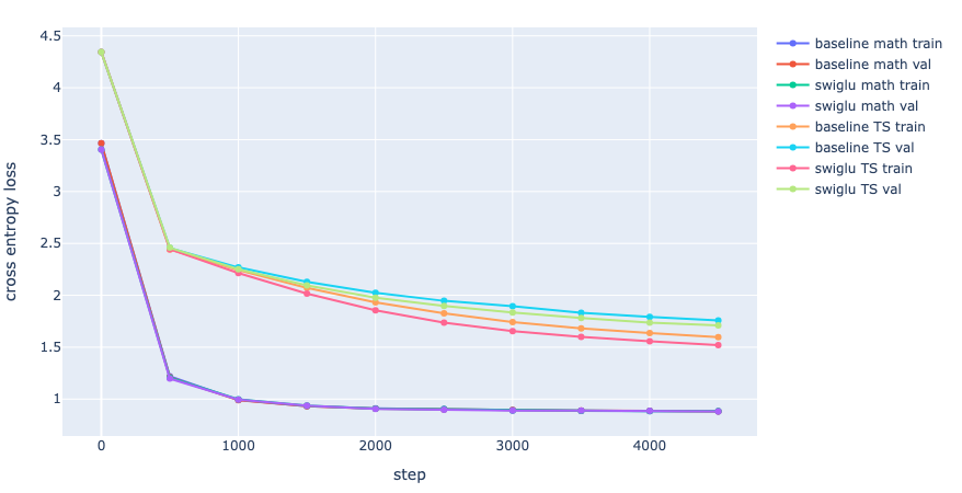
The training loss on TinyShakespeare decreased from 1.598 to 1.521, and the validation loss decreased from 1.758 to 1.711. Interestingly, there doesn’t seem to be an improvement in the final loss of our math dataset with the implementation of \(FNN_{SwiGLU}\). However, the starting loss is marginally better. This likely indicates that, at our current model size, the faster convergence provided by GLU isn’t effective in improving the performance of transformers for simple arithmetic tasks.
Summary
In summary, our exploration into enhancing transformer architectures with modern activation functions like SwiGLU reveals intriguing insights into their potential impact on model performance. While our experiments showcase improvements in convergence speed for certain tasks, they also underscore the nuanced nature of these enhancements, particularly in the context of arithmetic operations.